MATH325 Lab 5 Using Microsoft Excel to conduct ANOVA procedures The steps required for completing the deliverables for this assignment, including screen shots that correspond to these instructions, are outlined below. Complete the

MATH325 Lab 5

Using Microsoft Excel to conduct ANOVA procedures

The steps required for completing the deliverables for this assignment, including screen shots that correspond to these instructions, are outlined below. Complete the questions below and paste the answers from Excel below each question (type your answers to the questions where noted). Therefore, your response to the lab will be this ONE submitted document.

Context: Remember that statistics are far more than numbers or values – you need to know the context to perform a good analysis!

Study: A nurse practitioner is studying the effect of blood sugar (glucose) control, which involves collecting the average daily AC and QHS (fasting) blood sugar levels of the patients to determine if there is relationship between these and the patients’ Hemoglobin A1C level.  She hypothesizes that good blood sugar control will result in ideal Hemoglobin A1C levels and inadequate control of the patients’ blood sugar will result in high Hemoglobin A1C levels. 

She also tracks other factors that may contribute to the patients’ control of their blood sugar such as carbohydrate intake, age, frequency of glucose checks, and insurance coverage of diabetic supplies.

Hemoglobin: Ideal Hemoglobin A1C levels for patients are 6 or 7, a value of 8 or 9 merits concern, values 10 and up are considered severely uncontrolled, while values less than 6 are rare in diabetic patients.  4 and 5 can be found normally in patients that are not diabetic. 

Blood Sugar: Glucose levels under 70 are considered low, between 70 and 110 is considered normal, 111 to 170 is considered moderately high, and values above 170 are considered high. There is some debate on the cut points, however, these are the values used to categorize glucose levels in this study.

Glucose _Range: This is a categorical variable describing the group into which the patient’s glucose level places them: low, normal, moderately high, and high.

Glucose_Group: This is a numeric variable containing the same information as the Glucose_Range, however, the numeric value assigned to each group can be used in analysis that requires a ratio or interval level of measurement.  Low is assigned a 1, Normal is assigned a 2, Moderately High is assigned a 3, and High is assigned a 4.

Carbohydrates: Diabetic patients try to consume 14 servings of carbohydrates daily where each serving is approximately 15 grams.  This study tracks the average grams of carbohydrates consumed on a daily basis by these patients.

Age_Range: This is a Categorical Variable where each patient is classified by age: under 10, 11 – 16, 17 – 25, 26 – 40, 41 – 60, and over 60.

Age_Group: This is a numeric variable that contains the same information as the Age_Range, however, the numeric value assigned to each group can be used in analysis that requires a ratio or interval level of measurement.  Each patient is classified by age: under 10 is assigned a 0, 11 – 16 is assigned a 1, 17 – 25 is assigned a 2, 26 – 40 is assigned a 3, 41 – 60 is assigned a 4, and over 60 is assigned a 5.

Insurance: This is a categorical variable that describes if the patient’s insurance covers diabetic supplies.  Yes/No.

Insurance_Group: This is a numeric variable that describes the same information as the Insurance variable; however, the numeric value assigned to each group can be used in analysis that requires a ratio or interval level of measurement.  Yes is assigned a 1 and No is assigned a 0.

Frequency:  This numeric variable describes how many daily checks of their glucose level are typically performed on a given day for each diabetic patient.

 

 

Review the Microsoft Excel information on ANOVA: https://support.microsoft.com/en-us/office/use-the-analysis-toolpak-to-perform-complex-data-analysis-6c67ccf0-f4a9-487c-8dec-bdb5a2cefab6

Scroll down to ANOVA, and click to expand:

One of the first steps in the performance of an analysis of variance (ANOVA) is to validate the assumptions necessary for use of the test:

• Examine descriptive statistics for each of the independent variable’s groups and the Levene statistic to assess if the variances are equal.  The F statistic used in the ANOVA test can be robust to unequal variances if the samples sizes are approximately equal.  However, our first step is always to test the equality of the variances.
• It is also advisable to perform a plot of the means to get a visual indication of where you may expect to find similarities and differences among the groups.
• We will use Excel and request the descriptive statistics, and a plot of the Means (Box & Whisker) as well as calculate the F-Statistic with its significance.
• After the initial analysis, we will then perform an analysis using contrasts to target specific groups indicated by the data:
• Is there truly a difference between the low and normal groups?
• Is there a difference between the moderately high and high groups?
• Is there a difference between the normal and moderately high groups?

Then we perform the analysis.

To obtain a One-Way ANOVA using Microsoft Excel

1. Open the HealthCareData.xlsx file using Microsoft Excel.
2. First, we want to test the equality of the variances.  From the From Data Analysis menu, select F-Test Two-Sample for Variances. Click OK.

3. In the window that comes up, select the data under the Hemoglobin column for the Variable 1 Range, and the data under the Glucose_Group column for the Variable 2 Range.

4. Click OK to examine the output and perform an initial analysis of what you see.
5. To obtain the One-Way ANOVA, the variables that you are going to be investigating must be in adjacent columns. To get Hemoglobin and Glucose_Group aligned next to each other, insert a column next to one of the variables, and copy/paste the other variable into the newly-created column. From there, from the Data Analysis menu, select Anova: Single Factor. Click OK.

6. For the Input Range, select the two columns of data under the headers Hemoglobin and Glucose_Group. Note you will be selected both columns of data. Click OK.

 

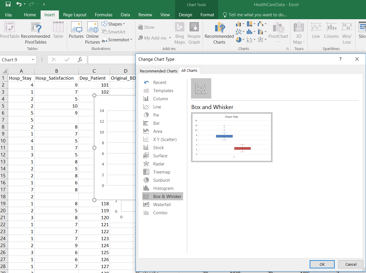
7. Create a Box Plot of the data as well. Highlight both columns of data and click Insert, Charts, Box & Whisker. Click OK.

8. Examine the output and compare it to the results from the Data Analysis output assessing Anova: Single Factor. Review the results.  This is the point at which you perform a contextual analysis of the output.
9. Think about it:  Were the assumptions for ANOVA met?  Can we proceed even if they aren’t?  Under what circumstances?  What did the data and tests show us about the two variables and the groups involved?

 

10. Deliverable: Save this document and submit it into the Assignments, Week 6: Lab.