MATH325 Lab 4 Using Microsoft Excel to Construct Linear Regression Models The steps required for completing the deliverables for this assignment, including screen shots that correspond to these instructions, are outlined be

 MATH325 Lab 4

Using Microsoft Excel to Construct Linear Regression Models

The steps required for completing the deliverables for this assignment, including screen shots that correspond to these instructions, are outlined below. Complete the questions below and paste the answers from Excel below each question (type your answers to the questions where noted). Therefore, your response to the lab will be this ONE submitted document.

Context: Remember that statistics are far more than numbers or values – you need to know the context to perform a good analysis!

Linear Regression.  Linear Regression estimates the coefficients of the linear equation, involving one or more independent variables that best predict the value of the dependent variable.  For example, you can try to predict a salesperson’s total yearly sales (the dependent variable) from independent variables such as age, education and years of experience.  Example.  Is the number of games won by a basketball team in a season related to the average number of points the team scores per game?  A scatter plot indicates that these variables are linearly related.  The number of games won and the average number of points scored by the opponent are also linearly related.  These variables have a negative relationship.  As the number of games won increases, the average number of points scored by the opponent decreases.  With linear regression, you can model the relationship of these variables.  A good model can be used to predict how many games teams will win.

Statistics.  For each variable: number of valid cases, mean, and standard deviation.  For each model: regression coefficients, correlation matrix, part and partial correlations, multiple R, R2, adjusted R2, standard error of the estimate, analysis-of-variance table, predicted values, and residuals.  Also, 95%-confidence intervals for each regression coefficient, variance-covariance matrix, variance inflation factor, tolerance, Durbin-Watson test, distance measures (Mahalanobis, Cook, and leverage values), DfBeta, DfFit, prediction intervals, and case-wise diagnostics.  Plots: scatter plots, partial plots, histograms, and normal probability plots.

For the purpose of testing hypotheses about the values of model parameters, the linear regression model also assumes the following:

1. The error term has a normal distribution with a mean of 0.
2. The variance of the error term is constant across cases and independent of the variables in the model.  An error term with non-constant variance is said to be heteroscedastic.
3. The value of the error term for a given case is independent of the values of the variables in the model and of the values of the error term for other cases.

Study: A nurse practitioner is studying the effect of blood sugar (glucose) control, which involves collecting the average daily AC and QHS (fasting) blood sugar levels of the patients to determine if there is a relationship between these and the patients’ Hemoglobin A1C level.  She hypothesizes that good blood sugar control will result in ideal Hemoglobin A1C levels and inadequate control of the patients’ blood sugar will result in high Hemoglobin A1C levels. 

She also tracks other factors that may contribute to the patients’ control of their blood sugar such as carbohydrate intake, age, frequency of glucose checks, and insurance coverage of diabetic supplies.  These will be analyzed in the next two labs.

Hemoglobin: Ideal Hemoglobin A1C levels are 6 to 7 whereas 8 or 9 merits concern and 10 and up are considered severely uncontrolled.  Values less than 6 are rare in diabetic patients.  However, levels lower than 6 can be found normally in patients that are not diabetic.

Blood Sugar: Glucose levels under 70 are considered low, between 70 and 110 is considered normal, 111 to 170 is considered moderately high, and values above 170 are considered high. There is some debate on the cutoff points, however, these are the values used to categorize glucose levels in this study.

Carbohydrates: Diabetic patients try to consume 14 servings of carbohydrates daily where each serving is approximately 15 grams.  This study tracks the average grams of carbohydrates consumed on a daily basis by these patients.

 

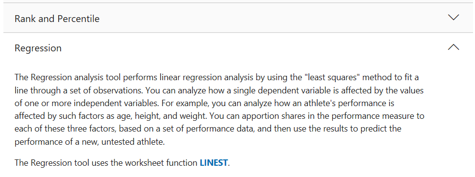
Review the Microsoft Excel information on Regression: https://support.microsoft.com/en-us/office/use-the-analysis-toolpak-to-perform-complex-data-analysis-6c67ccf0-f4a9-487c-8dec-bdb5a2cefab6

Scroll down to Regression, and click to expand:

To Obtain a Sample Scatter Plot Using Microsoft Excel

One of the first steps in the analysis of the study data is to create a scatter plot that compares the quantitative variables. Create each of the following scatter plots, find Pearson’s correlation coefficient, and perform the corresponding linear regression analysis in each case.  Detailed instructions follow on the next page.

• Create a scatter plot, find the r value, and perform the regression analysis that compares the patients’ average daily blood sugar level to their Hemoglobin A1C level.
• Create a scatter plot, find the r value, and perform the regression analysis that compares the patients’ carbohydrate intake to average glucose levels.
• Create a scatter plot, find the r value, and perform the regression analysis that compares the patients’ carbohydrate intake to Hemoglobin A1C levels.

 

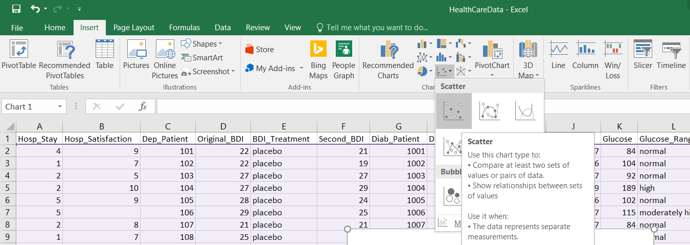
1. Open the HealthCareData.xlsx file using Excel.
2. From the menu, select Insert, and select Scatter from the scatterplot drop-down:
    A graph will automatically be created – do not worry, we will adjust accordingly. 

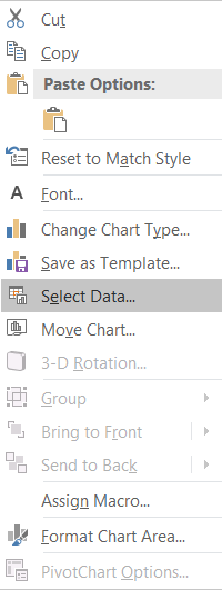
3. Right-click on the resulting graph, and from the menu that appears, click on Select Data:

4. Clear out the chart data range so that there is nothing there:

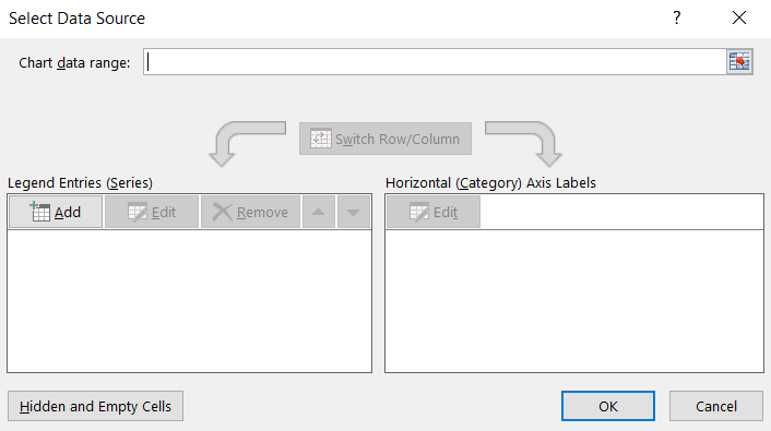
5. Under the Legend Entries (Series) area, click Add. In the window that opens:

 

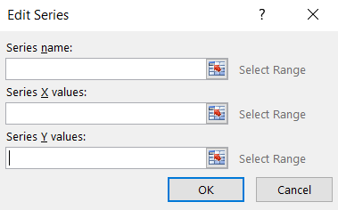
For the Series name, type in Glucose vs. Hemoglobin
 For the Series Y values, click on Select Range and highlight the Hemoglobin column.
 For the Series X values, click on Select Range and highlight the Glucose column.

Click OK.

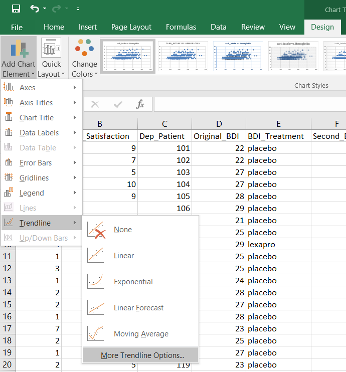
6. Examine the resulting graph. Click on the graph, and add a regression line. To do so, click on Design, Add Chart Element, Trendline, and More Trendline Options.

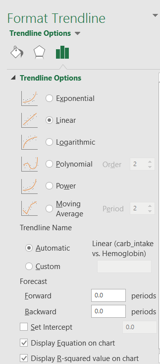
7. In the window that pops up, select the following and then click OK:

8. Examine the resulting graph.  Copy and paste it below.

 

9. Create two more graphs:

For the Series name, type in carb_intake vs. Glucose
 For the Series Y values, click on Select Range and highlight the Glucose column.
 For the Series X values, click on Select Range and highlight the carb_intake column.

For the Series name, type in carb_intake vs. Hemoglobin
 For the Series Y values, click on Select Range and highlight the Hemoglobin column.
 For the Series X values, click on Select Range and highlight the carb_intake column.

10. Examine the two additional graphs.  Copy and paste them below.

 

To Obtain Linear Regression Using Microsoft Excel

Calculating Regression in Hemoglobin levels versus Glucose levels

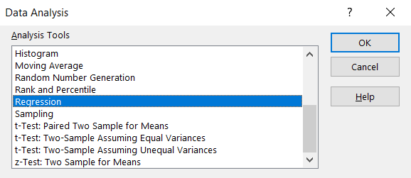
1. From Data Analysis menu, select Regression. Click OK.

1. In the window that pops up, select the following columns of data (not including the headers) for the Input Y Range and Input X Range:

• For the Series Y values, click on Select Range and highlight the Hemoglobin column.
• For the Series X values, click on Select Range and highlight the Glucose column.

Make sure that the following are checked:

11. Normal Probability Plots
12. Standardized Residuals

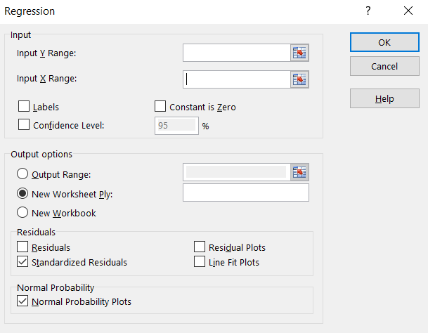
Click OK.

2. Copy and paste your results below (both the output table and plot). Think about it:  Was there a strong relationship indicated? Was there any extreme values that might skew results? How would you use the regression equations generated by the software?  Was the regression equation the same when calculated from the scatter plot as it was using the Data Analysis Toolpak? What preliminary conclusions would be supported and what further study indicated?

 

3. Repeat steps 1 and 2 for the studies that investigate carb_intake versus Glucose levels, and carb_intake versus Hemoglobin.
    

For the Series name, type in carb_intake vs. Glucose
 For the Series Y values, click on Select Range and highlight the Glucose column.
 For the Series X values, click on Select Range and highlight the carb_intake column.

 For the Series name, type in carb_intake vs. Hemoglobin
 For the Series Y values, click on Select Range and highlight the Hemoglobin column.
 For the Series X values, click on Select Range and highlight the carb_intake column.

 

4. Copy and paste your results for both studies below (both the output tables and plots). Think about it:  Were there strong relationships indicated? Were there any extreme values that might skew results? How would you use the regression equations generated by the software?  Were the regression equations the same when calculated from the scatter plots as they were using the Data Analysis Toolpak? What preliminary conclusions would be supported and what further study indicated?

 

5. Deliverable: Save this document and submit it into the Assignments, Week 5: Lab.